第六讲
本讲只要讲解最小二乘法的含义以及处理方式,如高斯牛顿(GN)、列文伯格-马夸尔特法(L-M)等下降法策略
在ch6/gaussNewton.cpp中,手写GN法,最小二乘估计曲线参数
//求解误差项
    for (int i = 0; i < N; i++) {
  double xi = x_data[i], yi = y_data[i];  // 第i个数据点
  double error = yi - exp(ae * xi * xi + be * xi + ce);
  Vector3d J; // 雅可比矩阵
  J[0] = -xi * xi * exp(ae * xi * xi + be * xi + ce);  // de/da
  J[1] = -xi * exp(ae * xi * xi + be * xi + ce);  // de/db
  J[2] = -exp(ae * xi * xi + be * xi + ce);  // de/dc

  H += inv_sigma * inv_sigma * J * J.transpose();
  b += -inv_sigma * inv_sigma * error * J;

  cost += error * error;
}

// 求解线性方程 Hx=b
//对于正定矩阵,可以使用cholesky分解来解方程
Vector3d dx = H.ldlt().solve(b);

//也可以使用QR分解
Vector3d dx = H.colPivHouseholderQr().solve(b);
ch6/ceresCurveFitting.cpp
使用ceres拟合曲线
// 代价函数的计算模型,结构体
struct CURVE_FITTING_COST {
  CURVE_FITTING_COST(double x, double y) : _x(x), _y(y) {}//构造函数初始化方式,给_x赋值x,_y赋值y

  // 残差的计算
  template<typename T>//函数模板
  bool operator()(          //括号运算符重载
    const T *const abc, // 模型参数,有3维
    T *residual) const {
    residual[0] = T(_y) - ceres::exp(abc[0] * T(_x) * T(_x) + abc[1] * T(_x) + abc[2]); // y-exp(ax^2+bx+c)
    return true;
  }

  const double _x, _y;    // x,y数据
};

  // 构建最小二乘问题
  ceres::Problem problem;
  for (int i = 0; i < N; i++) {
    problem.AddResidualBlock(     // 向问题中添加误差项
      // 使用自动求导,模板参数:误差类型,输出维度,输入维度,维数要与前面struct中一致
      new ceres::AutoDiffCostFunction<CURVE_FITTING_COST, 1, 3>(
        new CURVE_FITTING_COST(x_data[i], y_data[i])
      ),
      nullptr,            // 核函数,这里不使用,为空
      abc                 // 待估计参数
    );
  }


  // 配置求解器
  ceres::Solver::Options options;     // 这里有很多配置项可以填
  options.linear_solver_type = ceres::DENSE_NORMAL_CHOLESKY;  // 增量方程如何求解
  options.minimizer_progress_to_stdout = true;   // 输出到cout

  ceres::Solver::Summary summary;                // 优化信息
  chrono::steady_clock::time_point t1 = chrono::steady_clock::now();
  ceres::Solve(options, &problem, &summary);  // 开始优化
  chrono::steady_clock::time_point t2 = chrono::steady_clock::now();
  chrono::duration<double> time_used = chrono::duration_cast<chrono::duration<double>>(t2 - t1);
  cout << "solve time cost = " << time_used.count() << " seconds. " << endl;
ch6/g2oCurveFitting.cpp
待更新
第七讲
视觉里程计1,vo,特征提取与匹配,对极几何,PnP,ICP,三角化,BA,SVD,直接法,光流法,光度误差
ch7/orb_cv.cpp
#include <iostream>
#include <opencv2/core/core.hpp>
#include <opencv2/features2d/features2d.hpp>
#include <opencv2/highgui/highgui.hpp>
#include <chrono>
using namespace std;
using namespace cv;
int main(int argc, char **argv) {
if (argc != 3) {
cout << "usage: feature_extraction img1 img2" << endl;
return 1;
}
//-- 读取图像
Mat img_1 = imread(argv[1], CV_LOAD_IMAGE_COLOR);
Mat img_2 = imread(argv[2], CV_LOAD_IMAGE_COLOR);
assert(img_1.data != nullptr && img_2.data != nullptr);
//-- 初始化
std::vector<KeyPoint> keypoints_1, keypoints_2;
Mat descriptors_1, descriptors_2;
Ptr<FeatureDetector> detector = ORB::create(); //ORB
Ptr<DescriptorExtractor> descriptor = ORB::create();
Ptr<DescriptorMatcher> matcher = DescriptorMatcher::create("BruteForce-Hamming");
//-- 第一步:检测 Oriented FAST 角点位置
chrono::steady_clock::time_point t1 = chrono::steady_clock::now();
detector->detect(img_1, keypoints_1);
detector->detect(img_2, keypoints_2);
//-- 第二步:根据角点位置计算 BRIEF 描述子
descriptor->compute(img_1, keypoints_1, descriptors_1);
descriptor->compute(img_2, keypoints_2, descriptors_2);
chrono::steady_clock::time_point t2 = chrono::steady_clock::now();
chrono::duration<double> time_used = chrono::duration_cast<chrono::duration<double>>(t2 - t1);
cout << "extract ORB cost = " << time_used.count() << " seconds. " << endl;
Mat outimg1,outimg2;
drawKeypoints(img_1, keypoints_1, outimg1, Scalar::all(-1), DrawMatchesFlags::DEFAULT);
drawKeypoints(img_2, keypoints_2, outimg2, Scalar::all(-1), DrawMatchesFlags::DEFAULT);
imshow("pic1_ORB features", outimg1);
imshow("pic2_ORB features", outimg2);
//-- 第三步:对两幅图像中的BRIEF描述子进行匹配,使用 Hamming 距离
vector<DMatch> matches;
t1 = chrono::steady_clock::now();
matcher->match(descriptors_1, descriptors_2, matches);
t2 = chrono::steady_clock::now();
time_used = chrono::duration_cast<chrono::duration<double>>(t2 - t1);
cout << "match ORB cost = " << time_used.count() << " seconds. " << endl;
//-- 第四步:匹配点对筛选
// 计算最小距离和最大距离
auto min_max = minmax_element(matches.begin(), matches.end(),
[](const DMatch &m1, const DMatch &m2) { return m1.distance < m2.distance; });
double min_dist = min_max.first->distance;
double max_dist = min_max.second->distance;
printf("-- Max dist : %f \n", max_dist);
printf("-- Min dist : %f \n", min_dist);
//当描述子之间的距离大于两倍的最小距离时,即认为匹配有误.但有时候最小距离会非常小,设置一个经验值30作为下限.
std::vector<DMatch> good_matches;
for (int i = 0; i < descriptors_1.rows; i++) {
if (matches[i].distance <= max(2 * min_dist, 30.0)) {
good_matches.push_back(matches[i]);
}
}
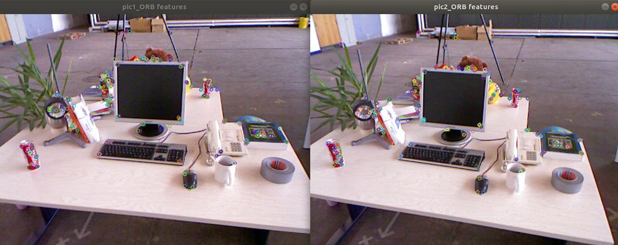
//-- 第五步:绘制匹配结果
Mat img_match;
Mat img_goodmatch;
drawMatches(img_1, keypoints_1, img_2, keypoints_2, matches, img_match);
drawMatches(img_1, keypoints_1, img_2, keypoints_2, good_matches, img_goodmatch);
imshow("all matches", img_match);
imshow("good matches", img_goodmatch);
waitKey(0);
return 0;
}
C++ Algorithm minmax_element()用法及代码示例
ch7/orb_self.cpp
手写ORB特征
(1)FAST角点检测
opencv库函数:利用ORB特征检测器detector里的detect函数。
手写:利用改进的FAST算法,增加了中心像素和围绕该像素的圆的像素之间的强度差阈值以及非最大值抑制。
其中的FAST()函数结构如下:
CV_EXPORTS void FAST( InputArray image, CV_OUT std::vector<KeyPoint>& keypoints,
                      int threshold, bool nonmaxSuppression=true );
/*
image: 检测的灰度图像
keypoints: 在图像上检测到的关键点
threshold: 中心像素和围绕该像素的圆的像素之间的强度差阈值
nonmaxSuppression: 参数非最大值抑制,默认为真,对检测到的角点应用非最大值抑制。
*/
(2)描述子计算
opencv库函数:构建ORB特征描述器descriptor里的compute函数
手写:自定义函数ComputeORB()来计算描述子,在这个函数里面首先会排除一些靠近边缘的特征点。排除的坏点的判断方式如下:
当kp.pt.x < half_boundary时,边长为boundary的图像块将在-x轴上超出图像。
当kp.pt.y < half_boundary时,边长为boundary的图像块将在-y轴上超出图像。
当kp.pt.x >= img.cols - half_boundary(kp.pt.x>= 640-16)时,边长为boundary(32)的图像块将在+x轴上超出图像。
当kp.pt.y >= img.rows - half_boundary(kp.pt.y>= 480-16)时,边长为boundary(32)的图像块将在+y轴上超出图像。
同时,在手写代码中,按照灰度质心法定义了图像块的矩和质心,最后求出了特征点的角度。
在求描述子时,事先准备了256*4个数据集,这些数据集表示以关键点为中心,[-13,12]的范围内,随机选点对p,q。选取两个点p,q,这两个点的坐标从数据集选取,然后乘上之前求的角度再加上关键点,以此找到关键点附近的两个随机像素,然后比较像素值。最终形成描述子。
(3)BRIEF描述子匹配函数
opencv下:利用自带的match函数,比较两副图像的描述子的汉明距离,并从小到大排序在matches容器中,然后在容器中挑选好的描述子,这些描述子满足描述子之间的距离小于两倍的最小距离和经验阈值的最小值,因为最小距离可能是0;
手写:描述子是采用256位二进制描述,对应到8个32位的unsigned int 数据,并利用SSE指令集计算每个unsigned int变量中1的个数,从而计算汉明距离。手写的暴力匹配代码中输入三个参数,分别是第一副和第二副图像的描述子,和存放输出匹配对的容器;这里的暴力匹配的思路为:取第一副图片中的一个描述子,分别计算与第二副图片每个描述子的汉明距离,然后选取最近的距离以及所对应的匹配对,然后多次选取图片1中的描述子重复上述操作,分别找到最短距离和相应的匹配对。最后再将比较得到的最小距离与设定的经验阈值作比较,如果小于经验阈值则保留并输出该匹配对。
具体代码如下:
// compute the descriptor
//(1)计算角点的方向;(2)计算描述子。
void ComputeORB(const cv::Mat &img, vector<cv::KeyPoint> &keypoints, vector<DescType> &descriptors) {
const int half_patch_size = 8; //计算特征点方向时,选取的图像块,16*16
const int half_boundary = 16;//计算描述子时在32*32的图像块中选点
int bad_points = 0; //计算描述子时,在32*32的区域块选择两个点比较,所选择的点超出图像范围的。出现这种情况下的FAST角点的数目。
//遍历所有FAST角点
for (auto &kp: keypoints)
{
//超出图像边界的角点的描述子设为空
if (kp.pt.x < half_boundary || kp.pt.y < half_boundary ||
kp.pt.x >= img.cols - half_boundary || kp.pt.y >= img.rows - half_boundary) {
// outside
bad_points++; //bad_points的描述子设为空
descriptors.push_back({});
continue;
}
//计算16*16图像块的灰度质心
//可参照下面的图片帮助理解
float m01 = 0, m10 = 0;//图像块的矩 视觉slam十四讲中p157
for (int dx = -half_patch_size; dx < half_patch_size; ++dx)
{
for (int dy = -half_patch_size; dy < half_patch_size; ++dy)
{
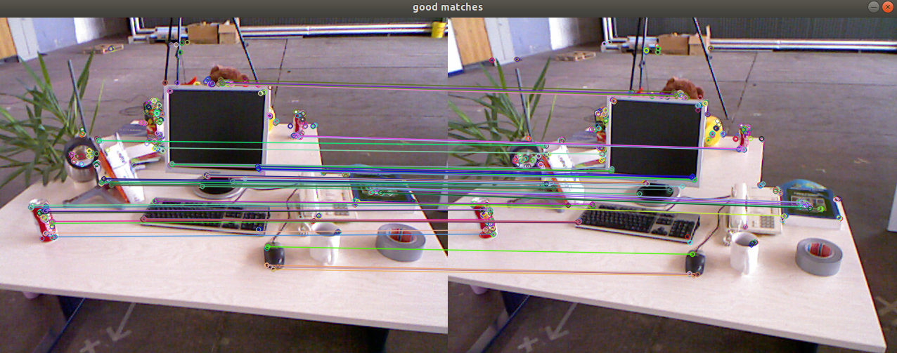
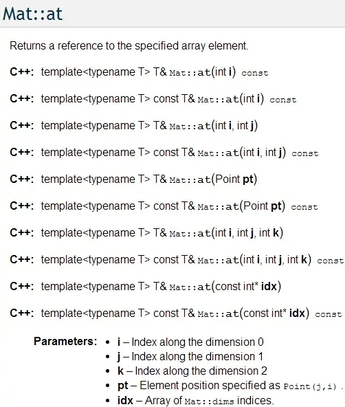
uchar pixel = img.at<uchar>(kp.pt.y + dy, kp.pt.x + dx);
m10 += dx * pixel; //pixel表示灰度值 视觉slam十四讲中p157最上面的公式
m01 += dy * pixel;//pixel表示灰度值 视觉slam十四讲中p157最上面的公式
}
}
// angle should be arc tan(m01/m10);参照下面第三章图片帮助理解
float m_sqrt = sqrt(m01 * m01 + m10 * m10) + 1e-18; // avoid divide by zero 1e-18避免了m_sqrt的值为0(图像块全黑)将m01 * m01 + m10 * m10进行开根
float sin_theta = m01 / m_sqrt;//sin_theta = m01 / 根号下(m01 * m01 + m10 * m10))
float cos_theta = m10 / m_sqrt;//cos_theta = m10 / 根号下(m01 * m01 + m10 * m10))
//因为tan_theta = m01/m10 即为tan_theta = sin_theta / cos_theta = [m01 / 根号下(m01 * m01 + m10 * m10] / [m10 / 根号下(m01 * m01 + m10 * m10]
//目的是求出特征点的方向 视觉slam十四讲中p157第三个公式
// compute the angle of this point
DescType desc(8, 0); //8个元素,它们的值初始化为0
for (int i = 0; i < 8; i++) {
uint32_t d = 0;
for (int k = 0; k < 32; k++)
{
int idx_pq = i * 32 + k;//idx_pq表示二进制描述子中的第几位
cv::Point2f p(ORB_pattern[idx_pq * 4], ORB_pattern[idx_pq * 4 + 1]);
cv::Point2f q(ORB_pattern[idx_pq * 4 + 2], ORB_pattern[idx_pq * 4 + 3]);
// rotate with theta
//p,q绕原点旋转theta得到pp,qq
cv::Point2f pp = cv::Point2f(cos_theta * p.x - sin_theta * p.y, sin_theta * p.x + cos_theta * p.y)
+ kp.pt;
cv::Point2f qq = cv::Point2f(cos_theta * q.x - sin_theta * q.y, sin_theta * q.x + cos_theta * q.y)
+ kp.pt;
if (img.at<uchar>(pp.y, pp.x) < img.at<uchar>(qq.y, qq.x)) {
d |= 1 << k;
}
}
desc[i] = d;
}
descriptors.push_back(desc);//desc表示该Oriented_FAST角点的描述子
}
cout << "bad/total: " << bad_points << "/" << keypoints.size() << endl;
}
// brute-force matching
void BfMatch(const vector<DescType> &desc1, const vector<DescType> &desc2, vector<cv::DMatch> &matches) {
const int d_max = 40;//描述子之间的距离小于这个值,才被认为是正确匹配
for (size_t i1 = 0; i1 < desc1.size(); ++i1) //size_t相当于int,便于代码移植
{
if (desc1[i1].empty()) continue;
cv::DMatch m{i1, 0, 256}; //定义了一个匹配对m
for (size_t i2 = 0; i2 < desc2.size(); ++i2)//计算描述子desc1[i1]和描述子desc2[i2]的距离,即不同位数的数目
{
if (desc2[i2].empty()) continue;
int distance = 0;
for (int k = 0; k < 8; k++) {
distance += _mm_popcnt_u32(desc1[i1][k] ^ desc2[i2][k]);
}
if (distance < d_max && distance < m.distance) {
m.distance = distance;
m.trainIdx = i2;
}
}
if (m.distance < d_max) {
matches.push_back(m);
}
}
ch7/pose_estimation_2d2d.cpp
本程序演示了如何使用2D-2D的特征匹配估计相机运动,对极约束求解相机运动
//
//
#include <iostream>
#include <opencv2/core/core.hpp>
#include <opencv2/features2d/features2d.hpp>
#include <opencv2/highgui/highgui.hpp>
#include <opencv2/calib3d/calib3d.hpp>

using namespace std;
using namespace cv;
//声明特征匹配函数
void find_feature_matches(const Mat &img1,const Mat &img2,
                          std::vector<KeyPoint> &keypoints_1,
                          std::vector<KeyPoint> &keypoints_2,
                          std::vector<DMatch> &matches);

//声明位姿估计函数
void pose_estimated_2d2d( std::vector<KeyPoint> keypoints_1,
                          std::vector<KeyPoint> keypoints_2,
                          std::vector<DMatch> matches,
                          Mat &R, Mat &t);

//声明 像素坐标转归一化坐标 p99页 公式5.5 变换一下就好啦!
//这里的函数我改了一下,书上的只是得到二维点,主程序中,还把二维点转换为三维点,我觉得多此一举,一个函数实现不就好了么
//下面是我实现的坐标变换函数 返回的是Mat类型,其实照片也是矩阵
Mat pixel2cam(const Point2d &p,const Mat &K);//p是像素坐标,K是相机内参矩阵

int main(int argc,char** argv)
{
    //运行可执行文件+图片1的路径+图片2的路径
    if(argc!=3)
    {
        cout<<"usage: ./pose_estimated_2d2d img1 img2"<<endl;
        return 1;
    }
    /*argv[1]="/home/nnz/data/slam_pratice/pratice_pose_estimated/1.png";
    argv[2]="/home/nnz/data/slam_pratice/pratice_pose_estimated/2.png";*/
    //读取图片
    Mat img1=imread(argv[1],CV_LOAD_IMAGE_COLOR);//彩色图
    Mat img2=imread(argv[2],CV_LOAD_IMAGE_COLOR);
    //定义要用到的变量啊,比如 keypoints_1,keypoints_2,matches
    vector<KeyPoint> keypoints_1, keypoints_2;
    vector<DMatch> matches;
    //计算两个keypoints的matches
    find_feature_matches(img1,img2,keypoints_1,keypoints_2,matches);
    //这样就得到matche啦!
    cout << "一共找到了" << matches.size() << "组匹配点" << endl;
    //重点来了
    //估计两组图片之间的运动
    Mat R,t;//定义一下旋转和平移
    pose_estimated_2d2d(keypoints_1,keypoints_2,matches,R,t);
    //这样就算出R ,t啦
    //当然我们还需要验证一下对极约束 准不准了
    //验证 E=t^R*scale;
    //t_x是t的反对称矩阵
    Mat t_x =
            (Mat_<double>(3, 3) << 0, -t.at<double>(2, 0), t.at<double>(1, 0),
                    t.at<double>(2, 0), 0, -t.at<double>(0, 0),
                    -t.at<double>(1, 0), t.at<double>(0, 0), 0);

    cout << "t^R=" << endl << t_x * R << endl;
    //验证对极约束 对应P167 页公式7.10 x2TEx1=0  E=t^*R
    //定义内参矩阵
    Mat K = (Mat_<double>(3, 3) << 520.9, 0, 325.1,
                                                 0, 521.0,249.7,
                                                 0, 0, 1);
    for(DMatch m: matches)
    {
        Mat x1=pixel2cam(keypoints_1[m.queryIdx].pt,K);
        Mat x2=pixel2cam(keypoints_2[m.queryIdx].pt,K);
        Mat d=x2.t()*t_x*R*x1;//若d很趋近于零,则说明没啥问题
        cout << "epipolar constraint = " << d << endl;
    }
    return 0;

}
//最复杂的地方来咯
//函数的实现
//匹配函数
void find_feature_matches(const Mat &img1,const Mat &img2,
                          std::vector<KeyPoint> &keypoints_1,
                          std::vector<KeyPoint> &keypoints_2,
                          std::vector<DMatch> &matches)
{
    //先初始化,创建咱们要用到的对象
    //定义两个关键点对应的描述子,同时创建检测keypoints的检测器
    Mat descriptors_1, descriptors_2;
    vector<DMatch> match;//暂时存放匹配点,因为后面还要进行筛选
    Ptr<FeatureDetector> detector=ORB::create();//keypoints检测器
    Ptr<DescriptorExtractor> descriptor =ORB::create();//描述子提取器
    Ptr<DescriptorMatcher> matcher =DescriptorMatcher::create(
            "BruteForce-Hamming");//描述子匹配器(方法:暴力匹配)
    //step1:找到角点
    detector->detect(img1,keypoints_1);//得到图1的关键点(keypoints_1)
    detector->detect(img2,keypoints_2);//得到图2的关键点(keypoints_2)
    //step2:计算关键点所对应的描述子
    descriptor->compute(img1,keypoints_1,descriptors_1);//得到descriptors_1
    descriptor->compute(img2,keypoints_2,descriptors_2);//得到descriptors_2
    //step3:进行暴力匹配
    matcher->match(descriptors_1,descriptors_2,match);
    //step4:对match进行筛选,得到好的匹配点,把好的匹配点放在matches中
    //先定义两个变量,一个是最大距离,一个是最小距离
    double min_dist=1000, max_dist=0;
    //找出所有匹配之间的最小距离和最大距离, 即是最相似的和最不相似的两组点之间的距离
    for(int i=0;i<descriptors_1.rows;i++) //描述子本质是由 0,1 组成的向量
    {
        double dist =match[i].distance;
        //还记得orb_cv中如何找最大距离和最远距离的吗,那里面的程序是用下面的函数实现的,下面的函数得到的是pair first 里面是最小距离,second里面是最大距离
        // minmax_element(matches.begin(),matched.end,[](const DMatch &m1,const DMatch &m2){return m1.distance<m2.distance;});
        //本程序用下面的if语句得到距离
        if (dist < min_dist) min_dist = dist;
        if (dist > max_dist) max_dist = dist;
    }
    printf("-- Max dist : %f \n", max_dist);
    printf("-- Min dist : %f \n", min_dist);
    //当描述子之间的距离大于两倍的最小距离时,即认为匹配有误.
    // 但有时候最小距离会非常小,设置一个经验值30作为下限.
    for(int i=0;i<descriptors_1.rows;i++)
    {
        if(match[i].distance<=max(2*min_dist,30.0))
        {
            matches.push_back(match[i]);
        }
    }
}
//像素到归一化坐标
Mat pixel2cam(const Point2d &p,const Mat &K)//p是像素坐标,K是相机内参矩阵
{
    Mat t;
    t=(Mat_<double>(3,1)<<(p.x - K.at<double>(0, 2)) / K.at<double>(0, 0),
            (p.y - K.at<double>(1, 2)) / K.at<double>(1, 1),1);
    return t;
}

//实现位姿估计函数
void pose_estimated_2d2d( std::vector<KeyPoint> keypoints_1,
                          std::vector<KeyPoint> keypoints_2,
                          std::vector<DMatch> matches,
                          Mat &R, Mat &t)
{
    // 相机内参来源于 TUM Freiburg2
    Mat K = (Mat_<double>(3, 3) << 520.9, 0, 325.1,
                                                 0, 521.0, 249.7,
                                                 0, 0, 1);

    //咱们要把关键点的像素点拿出来 ,定义两个容器接受两个图关键点的像素位置
    vector<Point2d> points1;
    vector<Point2d> points2;
    for(int i=0;i<(int)matches.size();i++)
    {
        //queryIdx是图1中匹配的关键点的对应编号
        //trainIdx是图2中匹配的关键点的对应编号
        //pt可以把关键点的像素位置取出来
        points1.push_back(keypoints_1[matches[i].queryIdx].pt);
        points2.push_back(keypoints_2[matches[i].trainIdx].pt);
    }
    //-- 计算基础矩阵
    Mat fundamental_matrix;
    fundamental_matrix = findFundamentalMat(points1, points2, CV_FM_8POINT);
    cout << "fundamental_matrix is " << endl << fundamental_matrix << endl;


    //计算本质矩阵 E
    //把cx ,cy放进一个向量里面 =相机的光心
    Point2d principal_point(325.1, 249.7);
    double focal_length=521;//相机的焦距
    //之所以取上面的principal_point、focal_length是因为计算本质矩阵的函数要用
    //得到本质矩阵essential_matrix
    Mat essential_matrix=findEssentialMat(points1,points2,focal_length,principal_point);
    cout<<" essential_matrix =\n"<< essential_matrix <<endl;

    //-- 计算单应矩阵 homography_matrix
    //-- 但是本例中场景不是平面,单应矩阵意义不大
    Mat homography_matrix;
    homography_matrix = findHomography(points1, points2, RANSAC, 3);
    cout << "homography_matrix is " << endl << homography_matrix << endl;
    //通过本质矩阵恢复咱们的 R  t
    recoverPose(essential_matrix,points1,points2,R,t,focal_length,principal_point);
    //输出咱们的 R t
    cout<<" 得到图1到图2 的位姿变换:\n "<<endl;
    cout<<"R= \n"<< R <<endl;
    cout<<"t= \n"<< t <<endl;
}
SLAM十四讲-ch7(2)-位姿估计(包含2d-2d、3d-2d、3d-3d、以及三角化实现代码的注释)
ch7/triangulation.cpp
在上面的2d2d位姿估计的基础上,利用三角化来获得特征匹配点的深度信息(通过画图,验证三维点与特征点的重投影关系)
//
// Created by wenbo on 2020/11/3.
//
//该程序在pose_estimated_2d2d的基础上加上三角化,以求得匹配的特征点在世界下的三维点
//
//
#include <iostream>
#include <opencv2/opencv.hpp>
// #include "extra.h" // used in opencv2
using namespace std;
using namespace cv;
//声明特征匹配函数
void find_feature_matches(const Mat &img1,const Mat &img2,
                          std::vector<KeyPoint> &keypoints_1,
                          std::vector<KeyPoint> &keypoints_2,
                          std::vector<DMatch> &matches);

//声明位姿估计函数
void pose_estimated_2d2d( std::vector<KeyPoint> &keypoints_1,
                          std::vector<KeyPoint> &keypoints_2,
                          std::vector<DMatch> &matches,
                          Mat &R, Mat &t);

//声明 像素坐标转归一化坐标 p99页 公式5.5 变换一下就好啦!
//这里的函数我改了一下,书上的只是得到二维点,主程序中,还把二维点转换为三维点,我觉得多此一举,一个函数实现不就好了么
//下面是我实现的坐标变换函数 返回的是Mat类型,其实照片也是矩阵
Point2f pixel2cam(const Point2d &p, const Mat &K);//p是像素坐标,K是相机内参矩阵

//声明三角化函数
void triangulation(
        const vector<KeyPoint> &keypoint_1,
        const vector<KeyPoint> &keypoint_2,
        const std::vector<DMatch> &matches,
        const Mat &R, const Mat &t,
        vector<Point3d> &points
);

/// 作图用
inline cv::Scalar get_color(float depth) {
    float up_th = 50, low_th = 10, th_range = up_th - low_th;
    if (depth > up_th) depth = up_th;
    if (depth < low_th) depth = low_th;
    return cv::Scalar(255 * depth / th_range, 0, 255 * (1 - depth / th_range));
}

int main(int argc,char** argv)
{
    //运行可执行文件+图片1的路径+图片2的路径
    if(argc!=3)
    {
        cout<<"usage: ./triangulation img1 img2"<<endl;
        return 1;
    }

    //读取图片
    Mat img1=imread(argv[1],CV_LOAD_IMAGE_COLOR);//彩色图
    Mat img2=imread(argv[2],CV_LOAD_IMAGE_COLOR);
    //定义要用到的变量啊,比如 keypoints_1,keypoints_2,matches
    vector<KeyPoint> keypoints_1, keypoints_2;
    vector<DMatch> matches;
    //计算两个keypoints的matches
    find_feature_matches(img1,img2,keypoints_1,keypoints_2,matches);
    //这样就得到matches啦!
    cout << "一共找到了" << matches.size() << "组匹配点" << endl;
    //重点来了
    //估计两组图片之间的运动
    Mat R,t;//定义一下旋转和平移
    pose_estimated_2d2d(keypoints_1,keypoints_2,matches,R,t);
    //这样就算出R ,t啦

    //三角化
    //定义一个容器 points 用来存放特征匹配点在世界坐标系下的3d点
    vector<Point3d> points;
    triangulation(keypoints_1,keypoints_2,matches,R,t,points);
    //得到三维点

    //验证三维点与特征点的重投影关系
    Mat K = (Mat_<double>(3, 3) << 520.9, 0, 325.1,
                                                 0, 521.0, 249.7,
                                                 0, 0, 1);
    Mat img_plot1=img1.clone();
    Mat img_plot2=img2.clone();
    //利用循环找到图1和图2特征点在图上的位置,并圈出来
    for(int i=0;i<matches.size();i++)
    {
        //先画图1中特征点
        //在这里,为什么从一个世界坐标系下的3d点,就可以得到,图1相机坐标下的深度点呢?
        //我觉得是因为 图1的位姿: R是单位矩阵,t为0(在三角化函数中有写到) 所以可以把图1的相机坐标看成是世界坐标
        float  depth1=points[i].z;//取出图1各个特征点的深度信息
        cout<<"depth: "<<depth1<<endl;
        Point2d pt1_cam=pixel2cam(keypoints_1[matches[i].queryIdx].pt,K);
        cv::circle(img_plot1, keypoints_1[matches[i].queryIdx].pt, 2, get_color(depth1), 2);

        //画图2
        //得到图2坐标系下的3d点,得到图2的深度信息
        Mat pt2_trans=R*(Mat_<double>(3, 1) <<points[i].x,points[i].y,points[i].z)+t;
        float depth2 = pt2_trans.at<double>(2, 0);
        cv::circle(img_plot2, keypoints_2[matches[i].trainIdx].pt, 2, get_color(depth2), 2);
    }
//画图
    cv::imshow("img 1", img_plot1);
    cv::imshow("img 2", img_plot2);
    cv::waitKey();


    return 0;

}

void triangulation(
        const vector<KeyPoint> &keypoint_1,
        const vector<KeyPoint> &keypoint_2,
        const std::vector<DMatch> &matches,
        const Mat &R, const Mat &t,
        vector<Point3d> &points
)
{
    //定义图1在世界坐标系下的位姿
    Mat T1 = (Mat_<float>(3, 4) <<
                                1, 0, 0, 0,
                                0, 1, 0, 0,
                                0, 0, 1, 0);

    //定义图2在世界坐标系下的位姿
    Mat T2 = (Mat_<float>(3, 4) <<
                                R.at<double>(0, 0), R.at<double>(0, 1), R.at<double>(0, 2), t.at<double>(0, 0),
            R.at<double>(1, 0), R.at<double>(1, 1), R.at<double>(1, 2), t.at<double>(1, 0),
            R.at<double>(2, 0), R.at<double>(2, 1), R.at<double>(2, 2), t.at<double>(2, 0)
    );
    Mat K = (Mat_<double>(3, 3) << 520.9, 0, 325.1, 0, 521.0, 249.7, 0, 0, 1);
    //容器 pts_1、pts_2分别存放图1和图2中特征点对应的自己相机归一化坐标中的 x与 y
    vector<Point2f> pts_1,pts_2;
    for(DMatch m:matches)//这样的遍历写起来比较快
    {
        //将像素坐标变为相机下的归一化坐标
        pts_1.push_back(pixel2cam(keypoint_1[m.queryIdx].pt,K));
        pts_2.push_back(pixel2cam(keypoint_2[m.trainIdx].pt,K));
    }
    Mat pts_4d;
    cv::triangulatePoints(T1,T2,pts_1,pts_2,pts_4d);
    /*
    传入两个图像对应相机的变化矩阵,各自相机坐标系下归一化相机坐标,
    输出的3D坐标是齐次坐标,共四个维度,因此需要将前三个维度除以第四个维度以得到非齐次坐标xyz
    */
    //转换为非齐次坐标
    for(int i=0;i<pts_4d.cols;i++)//遍历所有的点,列数表述点的数量
    {
        //定义x来接收每一个三维点
        Mat x=pts_4d.col(i); //x为4x1维度
        x/=x.at<float>(3,0);//归一化
        Point3d p(x.at<float>(0, 0),
                  x.at<float>(1, 0),
                  x.at<float>(2, 0));
        points.push_back(p);//将图1测得的目标相对相机实际位置(Xc,Yc,Zc)存入points
    }

}
ch7/pose_estimation_3d2d.cpp
本程序使用Opencv的EPnP求解pnp问题,并手写了一个高斯牛顿法的PnP,然后调用g2o来求解
//
// Created by nnz on 2020/11/5.
//
//
// Created by nnz on 2020/11/4.
//
#include <iostream>
#include <opencv2/core/core.hpp>
#include <opencv2/features2d/features2d.hpp>
#include <opencv2/highgui/highgui.hpp>
#include <opencv2/calib3d/calib3d.hpp>
#include <Eigen/Core>
#include <g2o/core/base_vertex.h>
#include <g2o/core/base_unary_edge.h>
#include <g2o/core/sparse_optimizer.h>
#include <g2o/core/block_solver.h>
#include <g2o/core/solver.h>
#include <g2o/core/optimization_algorithm_gauss_newton.h>
#include <g2o/solvers/dense/linear_solver_dense.h>
#include <sophus/se3.hpp>
#include <chrono>
//该程序用了三种方法实现位姿估计
//第一种,调用cv的函数pnp求解 R ,t
//第二种,手写高斯牛顿进行位姿优化
//第三种,利用g2o进行位姿优化
using namespace std;
using namespace cv;

typedef vector<Eigen::Vector2d, Eigen::aligned_allocator<Eigen::Vector2d>> VecVector2d;//VecVector2d可以定义存放二维向量的容器
typedef vector<Eigen::Vector3d, Eigen::aligned_allocator<Eigen::Vector3d>> VecVector3d;//VecVector3d可以定义存放三维向量的容器

void find_feature_matches(
        const Mat &img_1, const Mat &img_2,
        std::vector<KeyPoint> &keypoints_1,
        std::vector<KeyPoint> &keypoints_2,
        std::vector<DMatch> &matches);

// 像素坐标转相机归一化坐标
Point2d pixel2cam(const Point2d &p, const Mat &K);

// BA by gauss-newton 手写高斯牛顿进行位姿优化
void bundleAdjustmentGaussNewton(
        const VecVector3d &points_3d,
        const VecVector2d &points_2d,
        const Mat &K,
        Sophus::SE3d &pose
);

//利用g2o优化pose
void bundleAdjustmentG2O(
        const VecVector3d &points_3d,
        const VecVector2d &points_2d,
        const Mat &K,
        Sophus::SE3d &pose);

int main(int argc ,char** argv)
{


    //读取图片
    if (argc != 5) {
        cout << "usage: pose_estimation_3d2d img1 img2 depth1 depth2" << endl;
        return 1;
    }
    //读取图片
    Mat img_1=imread(argv[1],CV_LOAD_IMAGE_COLOR);//读取彩色图
    Mat img_2=imread(argv[2],CV_LOAD_IMAGE_COLOR);
    assert(img_1.data && img_2.data && "Can Not load images!");//若读取的图片没有内容,就终止程序
    vector<KeyPoint> keypoints_1, keypoints_2;
    vector<DMatch> matches;
    find_feature_matches(img_1,img_2,keypoints_1,keypoints_2,matches);//得到两个图片的特征匹配点
    cout << "一共找到了" << matches.size() << "组匹配点" << endl;


    //建立3d点,把深度图信息读进来,构造三维点
    Mat d1 = imread(argv[3], CV_LOAD_IMAGE_UNCHANGED);       // 深度图为16位无符号数,单通道图像
    Mat K = (Mat_<double>(3, 3) << 520.9, 0, 325.1, 0, 521.0, 249.7, 0, 0, 1);
    vector<Point3d> pts_3d;//创建容器pts_3d存放3d点(图1对应的特征点的相机坐标下的3d点)
    vector<Point2d> pts_2d;//创建容器pts_2d存放图2的特征点
    for(DMatch m:matches)
    {
        //把对应的图1的特征点的深度信息拿出来
        ushort d = d1.ptr<unsigned short>(int(keypoints_1[m.queryIdx].pt.y))[int(keypoints_1[m.queryIdx].pt.x)];
        if(d==0) //深度有问题
            continue;
        float dd=d/5000.0;//用dd存放换算过尺度的深度信息
        Point2d p1=pixel2cam(keypoints_1[m.queryIdx].pt,K);//p1里面放的是图1特征点在相机坐标下的归一化坐标(只包含 x,y)
        pts_3d.push_back(Point3d(p1.x*dd,p1.y*dd,dd));//得到图1特征点在相机坐标下的3d坐标
        pts_2d.push_back(keypoints_2[m.trainIdx].pt);//得到图2特张点的像素坐标
    }

    cout<<"3d-2d pairs:"<< pts_3d.size() <<endl;//3d-2d配对个数得用pts_3d的size
    cout<<"使用cv求解 位姿"<<endl;
    cout<<"***********************************opencv***********************************"<<endl;
    chrono::steady_clock::time_point t1 = chrono::steady_clock::now();
    Mat r, t;
    //Mat()这个参数指的是畸变系数向量?
    solvePnP(pts_3d, pts_2d, K, Mat(), r, t, false); // 调用OpenCV 的 PnP 求解,可选择EPNP,DLS等方法
    Mat R;
    cv::Rodrigues(r,R);//r是旋转向量,利用cv的Rodrigues()函数将旋转向量转换为旋转矩阵

    chrono::steady_clock::time_point t2 = chrono::steady_clock::now();
    chrono::duration<double> time_used = chrono::duration_cast<chrono::duration<double>>(t2 - t1);
    cout << "solve pnp in opencv cost time: " << time_used.count() << " seconds." << endl;

    cout << "R=" << endl << R << endl;
    cout << "t=" << endl << t << endl;
    cout<<"***********************************opencv***********************************"<<endl;
    cout<<"手写高斯牛顿优化位姿"<<endl;
    cout<<"***********************************手写高斯牛顿***********************************"<<endl;
    VecVector3d pts_3d_eigen;//存放3d点(图1对应的特征点的相机坐标下的3d点)
    VecVector2d pts_2d_eigen;//存放图2的特征点
    for(size_t i=0;i<pts_3d.size();i++)//size_t
    {
        pts_3d_eigen.push_back(Eigen::Vector3d(pts_3d[i].x,pts_3d[i].y,pts_3d[i].z));
        pts_2d_eigen.push_back(Eigen::Vector2d(pts_2d[i].x,pts_2d[i].y));
    }
    Sophus::SE3d pose_gn;//位姿(李群)
    t1 = chrono::steady_clock::now();
    bundleAdjustmentGaussNewton(pts_3d_eigen, pts_2d_eigen, K, pose_gn);
    t2 = chrono::steady_clock::now();
    time_used = chrono::duration_cast<chrono::duration<double>>(t2 - t1);
    cout << "solve pnp by gauss newton cost time: " << time_used.count() << " seconds." << endl;
    cout<<"R = \n"<<pose_gn.rotationMatrix()<<endl;
    cout<<"t = "<<pose_gn.translation().transpose()<<endl;
    cout<<"***********************************手写高斯牛顿***********************************"<<endl;

    cout<<"g2o优化位姿"<<endl;
    cout << "***********************************g2o***********************************" << endl;
    Sophus::SE3d pose_g2o;
    t1 = chrono::steady_clock::now();
    bundleAdjustmentG2O(pts_3d_eigen, pts_2d_eigen, K, pose_g2o);
    t2 = chrono::steady_clock::now();
    time_used = chrono::duration_cast<chrono::duration<double>>(t2 - t1);
    cout << "solve pnp by g2o cost time: " << time_used.count() << " seconds." << endl;
    cout << "***********************************g2o***********************************" << endl;
    return 0;

}
//实现特征匹配
void find_feature_matches(const Mat &img_1, const Mat &img_2,
                          std::vector<KeyPoint> &keypoints_1,
                          std::vector<KeyPoint> &keypoints_2,
                          std::vector<DMatch> &matches) {
    //-- 初始化
    Mat descriptors_1, descriptors_2;
    // used in OpenCV3
    Ptr<FeatureDetector> detector = ORB::create();
    Ptr<DescriptorExtractor> descriptor = ORB::create();
    // use this if you are in OpenCV2
    // Ptr<FeatureDetector> detector = FeatureDetector::create ( "ORB" );
    // Ptr<DescriptorExtractor> descriptor = DescriptorExtractor::create ( "ORB" );
    Ptr<DescriptorMatcher> matcher = DescriptorMatcher::create("BruteForce-Hamming");
    //-- 第一步:检测 Oriented FAST 角点位置
    detector->detect(img_1, keypoints_1);
    detector->detect(img_2, keypoints_2);

    //-- 第二步:根据角点位置计算 BRIEF 描述子
    descriptor->compute(img_1, keypoints_1, descriptors_1);
    descriptor->compute(img_2, keypoints_2, descriptors_2);

    //-- 第三步:对两幅图像中的BRIEF描述子进行匹配,使用 Hamming 距离
    vector<DMatch> match;
    // BFMatcher matcher ( NORM_HAMMING );
    matcher->match(descriptors_1, descriptors_2, match);

    //-- 第四步:匹配点对筛选
    double min_dist = 10000, max_dist = 0;

    //找出所有匹配之间的最小距离和最大距离, 即是最相似的和最不相似的两组点之间的距离
    for (int i = 0; i < descriptors_1.rows; i++) {
        double dist = match[i].distance;
        if (dist < min_dist) min_dist = dist;
        if (dist > max_dist) max_dist = dist;
    }

    printf("-- Max dist : %f \n", max_dist);
    printf("-- Min dist : %f \n", min_dist);

    //当描述子之间的距离大于两倍的最小距离时,即认为匹配有误.但有时候最小距离会非常小,设置一个经验值30作为下限.
    for (int i = 0; i < descriptors_1.rows; i++) {
        if (match[i].distance <= max(2 * min_dist, 30.0)) {
            matches.push_back(match[i]);
        }
    }
}

//实现像素坐标到相机坐标的转换(求出来的只是包含相机坐标下的x,y的二维点)
Point2d pixel2cam(const Point2d &p, const Mat &K) {
    return Point2d
            (
                    (p.x - K.at<double>(0, 2)) / K.at<double>(0, 0),
                    (p.y - K.at<double>(1, 2)) / K.at<double>(1, 1)
            );
}

//手写高斯牛顿
void bundleAdjustmentGaussNewton(
        const VecVector3d &points_3d,
        const VecVector2d &points_2d,
        const Mat &K,
        Sophus::SE3d &pose
)
{
    typedef Eigen::Matrix<double,6,1> Vector6d;
    const int iters=10;//迭代次数
    double cost=0,lastcost=0;//代价函数(目标函数)
    //拿出内参
    double fx = K.at<double>(0, 0);
    double fy = K.at<double>(1, 1);
    double cx = K.at<double>(0, 2);
    double cy = K.at<double>(1, 2);
    //进入迭代
    for (int iter = 0; iter <iters ; iter++)
    {
        Eigen::Matrix<double,6,6> H = Eigen::Matrix<double,6,6>::Zero();//初始化H矩阵
        Vector6d b = Vector6d::Zero();//对b矩阵初始化

        cost = 0;
        // 遍历所有的特征点  计算cost
        for(int i=0;i<points_3d.size();i++)
        {
            Eigen::Vector3d pc=pose*points_3d[i];//利用待优化的pose得到图2的相机坐标下的3d点
            double inv_z=1.0/pc[2];//得到图2的相机坐标下的3d点的z的倒数,也就是1/z
            double inv_z2 = inv_z * inv_z;//(1/z)^2
            //定义投影
            Eigen::Vector2d proj(fx * pc[0] / pc[2] + cx, fy * pc[1] / pc[2] + cy);
            //定义误差
            Eigen::Vector2d e=points_2d[i]-proj;
            cost += e.squaredNorm();//cost=e*e
            //定义雅克比矩阵J
            Eigen::Matrix<double, 2, 6> J;
            J << -fx * inv_z,
                    0,
                    fx * pc[0] * inv_z2,
                    fx * pc[0] * pc[1] * inv_z2,
                    -fx - fx * pc[0] * pc[0] * inv_z2,
                    fx * pc[1] * inv_z,
                    0,
                    -fy * inv_z,
                    fy * pc[1] * inv_z2,
                    fy + fy * pc[1] * pc[1] * inv_z2,
                    -fy * pc[0] * pc[1] * inv_z2,
                    -fy * pc[0] * inv_z;

            H += J.transpose() * J;
            b += -J.transpose() * e;
        }
        //出了这个内循环,表述结束一次迭代的计算,接下来,要求pose了
        Vector6d dx;//P129页 公式6.33 计算增量方程 Hdx=b
        dx = H.ldlt().solve(b);//算出增量dx
        //判断dx这个数是否有效
        if (isnan(dx[0]))
        {
            cout << "result is nan!" << endl;
            break;
        }
        //如果我们进行了迭代,且最后的cost>=lastcost的话,那就表明满足要求了,可以停止迭代了
        if (iter > 0 && cost >= lastcost)
        {
            // cost increase, update is not good
            cout << "cost: " << cost << ", last cost: " << lastcost << endl;
            break;
        }
        //优化pose 也就是用dx更新pose
        pose=Sophus::SE3d::exp(dx) * pose;//dx是李代数,要转换为李群
        lastcost=cost;
        cout << "iteration " << iter << " cost="<< std::setprecision(12) << cost << endl;
        //std::setprecision(12)浮点数控制位数为12位
        //如果误差特别小了,也结束迭代
        if (dx.norm() < 1e-6)
        {
            // converge
            break;
        }
    }
    cout<<"pose by g-n \n"<<pose.matrix()<<endl;
}

//对于用g2o来进行优化的话,首先要定义顶点和边的模板
//顶点,也就是咱们要优化的pose 用李代数表示它 6维
class Vertexpose: public g2o::BaseVertex<6,Sophus::SE3d>L
{
public:
    EIGEN_MAKE_ALIGNED_OPERATOR_NEW;//必须写,我也不知道为什么
    //重载setToOriginImpl函数 这个应该就是把刚开的待优化的pose放进去
    virtual void setToOriginImpl() override
    {
        _estimate = Sophus::SE3d();
    }
    //重载oplusImpl函数,用来更新pose(待优化的系数)
    virtual void oplusImpl(const double *update) override
    {
        Eigen::Matrix<double,6,1> update_eigen;//更新的量,就是增量呗,dx
        update_eigen << update[0], update[1], update[2], update[3], update[4], update[5];
        _estimate=Sophus::SE3d::exp(update_eigen)* _estimate;//更新pose 李代数要转换为李群,这样才可以左乘
    }
    //存盘 读盘 :留空
    virtual bool read(istream &in) override {}

    virtual bool write(ostream &out) const override {}
};
//定义边模板 边也就是误差,二维 并且把顶点也放进去
class EdgeProjection : public g2o::BaseUnaryEdge<2,Eigen::Vector2d,Vertexpose>
{
public:
    EIGEN_MAKE_ALIGNED_OPERATOR_NEW;//必须写,我也不知道为什么
    //有参构造,初始化 图1中的3d点 以及相机内参K
    EdgeProjection(const Eigen::Vector3d &pos, const Eigen::Matrix3d &K) : _pos3d(pos),_K(K) {}
    //计算误差
    virtual void computeError() override
    {
        const Vertexpose *v=static_cast<const Vertexpose *>(_vertices[0]);
        Sophus::SE3d T=v->estimate();
        Eigen::Vector3d pos_pixel = _K * (T * _pos3d);//T * _pos3d是图2的相机坐标下的3d点
        pos_pixel /= pos_pixel[2];//得到了像素坐标的齐次形式
        _error = _measurement - pos_pixel.head<2>();
    }
    //计算雅克比矩阵
    virtual void linearizeOplus() override
    {
        const Vertexpose *v = static_cast<Vertexpose *> (_vertices[0]);
        Sophus::SE3d T = v->estimate();
        Eigen::Vector3d pos_cam=T*_pos3d;//图2的相机坐标下的3d点
        double fx = _K(0, 0);
        double fy = _K(1, 1);
        double cx = _K(0, 2);
        double cy = _K(1, 2);
        double X = pos_cam[0];
        double Y = pos_cam[1];
        double Z = pos_cam[2];
        double Z2 = Z * Z;
        //雅克比矩阵见 书 p187 公式7.46
        _jacobianOplusXi
                << -fx / Z, 0, fx * X / Z2, fx * X * Y / Z2, -fx - fx * X * X / Z2, fx * Y / Z,
                0, -fy / Z, fy * Y / (Z * Z), fy + fy * Y * Y / Z2, -fy * X * Y / Z2, -fy * X / Z;


    }
    //存盘 读盘 :留空
    virtual bool read(istream &in) override {}

    virtual bool write(ostream &out) const override {}
private:
    Eigen::Vector3d _pos3d;
    Eigen::Matrix3d _K;
};


//利用g2o优化pose
void bundleAdjustmentG2O(
        const VecVector3d &points_3d,
        const VecVector2d &points_2d,
        const Mat &K,
        Sophus::SE3d &pose)
{
    // 构建图优化,先设定g2o
    typedef g2o::BlockSolver<g2o::BlockSolverTraits<6, 3>> BlockSolverType;  //  优化系数pose is 6, 数据点 landmark is 3
    typedef g2o::LinearSolverDense<BlockSolverType::PoseMatrixType> LinearSolverType; // 线性求解器类型
    // 梯度下降方法,可以从GN, LM, DogLeg 中选
    auto solver = new g2o::OptimizationAlgorithmGaussNewton(
            g2o::make_unique<BlockSolverType>
                    (g2o::make_unique<LinearSolverType>()));//把设定的类型都放进求解器

    g2o::SparseOptimizer optimizer;     // 图模型
    optimizer.setAlgorithm(solver);   // 设置求解器 算法g-n
    optimizer.setVerbose(true);       // 打开调试输出
    //加入顶点
    Vertexpose *v=new Vertexpose();
    v->setEstimate(Sophus::SE3d());
    v->setId(0);
    optimizer.addVertex(v);
    //K
    // K
    Eigen::Matrix3d K_eigen;
    K_eigen <<
            K.at<double>(0, 0), K.at<double>(0, 1), K.at<double>(0, 2),
            K.at<double>(1, 0), K.at<double>(1, 1), K.at<double>(1, 2),
            K.at<double>(2, 0), K.at<double>(2, 1), K.at<double>(2, 2);

    //加入边
    int index=1;
    for(size_t i=0;i<points_2d.size();++i)
    {
        //遍历 把3d点和像素点拿出来
        auto p2d = points_2d[i];
        auto p3d = points_3d[i];
        EdgeProjection *edge = new EdgeProjection(p3d, K_eigen);//有参构造
        edge->setId(index);
        edge->setVertex(0,v);
        edge->setMeasurement(p2d);//设置观测值,其实就是图2 里的匹配特征点的像素位置
        edge->setInformation(Eigen::Matrix2d::Identity());//信息矩阵是二维方阵,因为误差是二维
        optimizer.addEdge(edge);//加入边
        index++;//边的编号++
    }
    chrono::steady_clock::time_point t1 = chrono::steady_clock::now();
    optimizer.setVerbose(true);
    optimizer.initializeOptimization();//开始  初始化
    optimizer.optimize(10);//迭代次数
    chrono::steady_clock::time_point t2 = chrono::steady_clock::now();
    chrono::duration<double> time_used = chrono::duration_cast<chrono::duration<double>>(t2 - t1);
    cout << "optimization costs time: " << time_used.count() << " seconds." << endl;
    cout << "pose estimated by g2o =\n" << v->estimate().matrix() << endl;
    pose = v->estimate();

}
SLAM十四讲-ch7(2)-位姿估计(包含2d-2d、3d-2d、3d-3d、以及三角化实现代码的注释)
ch7/pose_estimation_3d3d.cpp
//
// Created by nnz on 2020/11/5.
//
#include <iostream>
#include <opencv2/core/core.hpp>
#include <opencv2/features2d/features2d.hpp>
#include <opencv2/highgui/highgui.hpp>
#include <opencv2/calib3d/calib3d.hpp>
#include <Eigen/Core>
#include <g2o/core/base_vertex.h>
#include <g2o/core/base_unary_edge.h>
#include <g2o/core/sparse_optimizer.h>
#include <g2o/core/block_solver.h>
#include <g2o/core/solver.h>
#include <g2o/core/optimization_algorithm_gauss_newton.h>
#include <g2o/solvers/dense/linear_solver_dense.h>
#include <sophus/se3.hpp>
#include <chrono>
using namespace std;
using namespace cv;

void find_feature_matches(
        const Mat &img_1, const Mat &img_2,
        std::vector<KeyPoint> &keypoints_1,
        std::vector<KeyPoint> &keypoints_2,
        std::vector<DMatch> &matches);

// 像素坐标转相机归一化坐标
Point2d pixel2cam(const Point2d &p, const Mat &K);

void pose_estimation_3d3d(
        const vector<Point3f> &pts1,
        const vector<Point3f> &pts2,
        Mat &R, Mat &t
);

//
void bundleAdjustment(
        const vector<Point3f> &pts1,
        const vector<Point3f> &pts2,
        Mat &R, Mat &t);
int main(int argc,char** argv)
{
    if(argc!=5)
    {
        cout<<" usage: pose_estimation_3d3d img1 img2 depth1 depth2 "<<endl;
        return 1;
    }
    //读取图片
    Mat img_1=imread(argv[1],CV_LOAD_IMAGE_COLOR);//读取彩色图
    Mat img_2=imread(argv[2],CV_LOAD_IMAGE_COLOR);
    vector<KeyPoint> keypoints_1, keypoints_2;//容器keypoints_1, keypoints_2分别存放图1和图2的特征点
    vector<DMatch> matches;
    find_feature_matches(img_1, img_2, keypoints_1, keypoints_2, matches);//得到图1与图2的特征匹配点
    cout << "一共找到了" << matches.size() << "组匹配点" << endl;
    //接下来的是建立3d点 利用深度图可以获取深度信息
    //depth1是图1对应的深度图 depth2是图2对应的深度图
    Mat depth1 = imread(argv[3], CV_LOAD_IMAGE_UNCHANGED);       // 深度图为16位无符号数,单通道图像
    Mat depth2 = imread(argv[4], CV_LOAD_IMAGE_UNCHANGED);

    //内参矩阵
    Mat K =(Mat_<double>(3, 3) << 520.9, 0, 325.1, 0, 521.0, 249.7, 0, 0, 1);
    vector<Point3f> pts1, pts2;

    for(DMatch m:matches)
    {
        //先把两图特征匹配点对应的深度拿出来
        ushort d1=depth1.ptr<unsigned short >(int(keypoints_1[m.queryIdx].pt.y))[int(keypoints_1[m.queryIdx].pt.x)];
        ushort d2=depth2.ptr<unsigned short >(int(keypoints_2[m.trainIdx].pt.y))[int(keypoints_2[m.trainIdx].pt.x)];
        if(d1==0 || d2==0)//深度无效
            continue;
        Point2d p1=pixel2cam(keypoints_1[m.queryIdx].pt,K);//得到图1的特征匹配点在其相机坐标下的x ,y
        Point2d p2=pixel2cam(keypoints_2[m.trainIdx].pt,K);//得到图2的特征匹配点在其相机坐标下的x ,y
        //对深度进行尺度变化得到真正的深度
        float dd1 = float(d1) / 5000.0;
        float dd2 = float(d2) / 5000.0;
        //容器 pts_1与pts_2分别存放 图1中的特征匹配点其相机坐标下的3d点 和 图2中的特征匹配点其相机坐标下的3d点
        pts1.push_back(Point3f(p1.x * dd1, p1.y * dd1, dd1));
        pts2.push_back(Point3f(p2.x * dd2, p2.y * dd2, dd2));
    }
    //这样就可以得到 3d-3d的匹配点
    cout << "3d-3d pairs: " << pts1.size() << endl;
    Mat R, t;
    cout<<" ************************************ICP 3d-3d by SVD**************************************** "<<endl;
    pose_estimation_3d3d(pts1, pts2, R, t);
    cout << "ICP via SVD results: " << endl;
    cout << "R = " << R << endl;
    cout << "t = " << t << endl;
    cout << "R^T = " << R.t() << endl;
    cout << "t^T = " << -R.t() * t << endl;
    cout<<" ************************************ICP 3d-3d by SVD**************************************** "<<endl;
    cout<<endl;
    cout<<" ************************************ICP 3d-3d by g2o**************************************** "<<endl;
    bundleAdjustment(pts1, pts2, R, t);
    cout<<"R= \n"<<R<<endl;
    cout<<"t = "<< t.t() <<endl;
    cout<<"验证 p2 = R*P1 +t "<<endl;
    for (int i = 0; i < 5; i++) {
        cout << "p1 = " << pts1[i] << endl;
        cout << "p2 = " << pts2[i] << endl;
        cout << "(R*p1+t) = " <<
             R * (Mat_<double>(3, 1) << pts1[i].x, pts1[i].y, pts1[i].z) + t
             << endl;
        cout << endl;
    }
    cout<<" ************************************ICP 3d-3d by g2o**************************************** "<<endl;

    return 0;
}

void find_feature_matches(const Mat &img_1, const Mat &img_2,
                          std::vector<KeyPoint> &keypoints_1,
                          std::vector<KeyPoint> &keypoints_2,
                          std::vector<DMatch> &matches) {
    //-- 初始化
    Mat descriptors_1, descriptors_2;
    // used in OpenCV3
    Ptr<FeatureDetector> detector = ORB::create();
    Ptr<DescriptorExtractor> descriptor = ORB::create();
    // use this if you are in OpenCV2
    // Ptr<FeatureDetector> detector = FeatureDetector::create ( "ORB" );
    // Ptr<DescriptorExtractor> descriptor = DescriptorExtractor::create ( "ORB" );
    Ptr<DescriptorMatcher> matcher = DescriptorMatcher::create("BruteForce-Hamming");
    //-- 第一步:检测 Oriented FAST 角点位置
    detector->detect(img_1, keypoints_1);
    detector->detect(img_2, keypoints_2);

    //-- 第二步:根据角点位置计算 BRIEF 描述子
    descriptor->compute(img_1, keypoints_1, descriptors_1);
    descriptor->compute(img_2, keypoints_2, descriptors_2);

    //-- 第三步:对两幅图像中的BRIEF描述子进行匹配,使用 Hamming 距离
    vector<DMatch> match;
    // BFMatcher matcher ( NORM_HAMMING );
    matcher->match(descriptors_1, descriptors_2, match);

    //-- 第四步:匹配点对筛选
    double min_dist = 10000, max_dist = 0;

    //找出所有匹配之间的最小距离和最大距离, 即是最相似的和最不相似的两组点之间的距离
    for (int i = 0; i < descriptors_1.rows; i++) {
        double dist = match[i].distance;
        if (dist < min_dist) min_dist = dist;
        if (dist > max_dist) max_dist = dist;
    }

    printf("-- Max dist : %f \n", max_dist);
    printf("-- Min dist : %f \n", min_dist);

    //当描述子之间的距离大于两倍的最小距离时,即认为匹配有误.但有时候最小距离会非常小,设置一个经验值30作为下限.
    for (int i = 0; i < descriptors_1.rows; i++) {
        if (match[i].distance <= max(2 * min_dist, 30.0)) {
            matches.push_back(match[i]);
        }
    }
}

//实现像素坐标到相机坐标的转换(求出来的只是包含相机坐标下的x,y的二维点)
Point2d pixel2cam(const Point2d &p, const Mat &K) {
    return Point2d
            (
                    (p.x - K.at<double>(0, 2)) / K.at<double>(0, 0),
                    (p.y - K.at<double>(1, 2)) / K.at<double>(1, 1)
            );
}

//参考书上的p197页
void pose_estimation_3d3d(
        const vector<Point3f> &pts1,
        const vector<Point3f> &pts2,
        Mat &R, Mat &t
)
{
    int N=pts1.size();//匹配的3d点个数
    Point3f p1,p2;//质心
    for(int i=0;i<N;i++)
    {
        p1+=pts1[i];
        p2+=pts2[i];
    }
    p1 = Point3f(Vec3f(p1)/N);//得到质心
    p2 = Point3f(Vec3f(p2) / N);
    vector<Point3f> q1(N),q2(N);
    for(int i=0;i<N;i++)
    {
        //去质心
        q1[i]=pts1[i]-p1;
        q2[i]=pts2[i]-p2;
    }
    //计算 W+=q1*q2^T(求和)
    Eigen::Matrix3d W=Eigen::Matrix3d::Zero();//初始化
    for(int i=0;i<N;i++)
    {
        W+= Eigen::Vector3d (q1[i].x,q1[i].y,q1[i].z)*(Eigen::Vector3d (q2[i].x,q2[i].y,q2[i].z).transpose());
    }
    cout<<"W = "<<endl<<W<<endl;
    //利用svd分解 W=U*sigema*V
    Eigen::JacobiSVD<Eigen::Matrix3d> svd(W,Eigen::ComputeFullU | Eigen::ComputeFullV);
    Eigen::Matrix3d U=svd.matrixU();//得到U矩阵
    Eigen::Matrix3d V=svd.matrixV();//得到V矩阵
    cout << "U=" << U << endl;
    cout << "V=" << V << endl;
    Eigen::Matrix3d R_=U*(V.transpose());
    if (R_.determinant() < 0)//若旋转矩阵R_的行列式<0 则取负号
    {
        R_ = -R_;
    }
    Eigen::Vector3d t_=Eigen::Vector3d (p1.x,p1.y,p1.z)-R_*Eigen::Vector3d (p2.x,p2.y,p2.z);//得到平移向量
    //把 Eigen形式的 r 和 t_ 转换为CV 中的Mat格式
    R = (Mat_<double>(3, 3) <<
                            R_(0, 0), R_(0, 1), R_(0, 2),
            R_(1, 0), R_(1, 1), R_(1, 2),
            R_(2, 0), R_(2, 1), R_(2, 2)
    );
    t = (Mat_<double>(3, 1) << t_(0, 0), t_(1, 0), t_(2, 0));
}

//对于用g2o来进行优化的话,首先要定义顶点和边的模板
//顶点,也就是咱们要优化的pose 用李代数表示它 6维
class Vertexpose: public g2o::BaseVertex<6,Sophus::SE3d>
{
public:
    EIGEN_MAKE_ALIGNED_OPERATOR_NEW;//必须写,我也不知道为什么
    //重载setToOriginImpl函数 这个应该就是把刚开的待优化的pose放进去
    virtual void setToOriginImpl() override
    {
        _estimate = Sophus::SE3d();
    }
    //重载oplusImpl函数,用来更新pose(待优化的系数)
    virtual void oplusImpl(const double *update) override
    {
        Eigen::Matrix<double,6,1> update_eigen;//更新的量,就是增量呗,dx
        update_eigen << update[0], update[1], update[2], update[3], update[4], update[5];
        _estimate=Sophus::SE3d::exp(update_eigen)* _estimate;//更新pose 李代数要转换为李群,这样才可以左乘
    }
    //存盘 读盘 :留空
    virtual bool read(istream &in) override {}

    virtual bool write(ostream &out) const override {}
};
//定义边
class EdgeProjectXYZRGBD: public g2o::BaseUnaryEdge<3,Eigen::Vector3d,Vertexpose>
{
public:
    EdgeProjectXYZRGBD(const Eigen::Vector3d &point) : _point(point) {}//赋值这个是图1坐标下的3d点
    //计算误差
    virtual void computeError() override
    {
        const Vertexpose *v=static_cast<const Vertexpose *>(_vertices[0]);//顶点v
        _error = _measurement - v->estimate() * _point;


    }
    //计算雅克比
    virtual void linearizeOplus() override
    {
        const Vertexpose *v=static_cast<const Vertexpose *>(_vertices[0]);//顶点v
        Sophus::SE3d T=v->estimate();//把顶点的待优化系数拿出来
        Eigen::Vector3d xyz_trans=T*_point;//变换到图2下的坐标点
        //下面的雅克比没看懂
        _jacobianOplusXi.block<3, 3>(0, 0) = -Eigen::Matrix3d::Identity();
        _jacobianOplusXi.block<3, 3>(0, 3) = Sophus::SO3d::hat(xyz_trans);

    }

    bool read(istream &in) {}

    bool write(ostream &out) const {}
protected:
    Eigen::Vector3d _point;
};
//利用g2o
void bundleAdjustment(const vector<Point3f> &pts1,
                      const vector<Point3f> &pts2,
                      Mat &R, Mat &t)
{
// 构建图优化,先设定g2o
    typedef g2o::BlockSolver<g2o::BlockSolverTraits<6, 3>> BlockSolverType;  //  优化系数pose is 6, 数据点 landmark is 3
    typedef g2o::LinearSolverDense<BlockSolverType::PoseMatrixType> LinearSolverType; // 线性求解器类型
    // 梯度下降方法,可以从GN, LM, DogLeg 中选
    auto solver = new g2o::OptimizationAlgorithmGaussNewton(
            g2o::make_unique<BlockSolverType>
                    (g2o::make_unique<LinearSolverType>()));//把设定的类型都放进求解器
    g2o::SparseOptimizer optimizer;     // 图模型
    optimizer.setAlgorithm(solver);   // 设置求解器 算法g-n
    optimizer.setVerbose(true);       // 打开调试输出
    //加入顶点
    Vertexpose *v=new Vertexpose();
    v->setEstimate(Sophus::SE3d());
    v->setId(0);
    optimizer.addVertex(v);

    //加入边
    int index=1;
    for(size_t i=0;i<pts1.size();i++)
    {
        EdgeProjectXYZRGBD *edge = new EdgeProjectXYZRGBD(Eigen::Vector3d(pts1[i].x,pts1[i].y,pts1[i].z));
        edge->setId(index);//边的编号
        edge->setVertex(0,v);//设置顶点  顶点编号
        edge->setMeasurement(Eigen::Vector3d(pts2[i].x,pts2[i].y,pts2[i].z));
        edge->setInformation(Eigen::Matrix3d::Identity());//set信息矩阵为单位矩阵
        optimizer.addEdge(edge);//加入边
        index++;
    }
    chrono::steady_clock::time_point t1 = chrono::steady_clock::now();
    optimizer.initializeOptimization();//开始
    optimizer.optimize(10);//迭代次数
    chrono::steady_clock::time_point t2 = chrono::steady_clock::now();
    chrono::duration<double> time_used = chrono::duration_cast<chrono::duration<double>>(t2 - t1);
    cout << "optimization costs time: " << time_used.count() << " seconds." << endl;

    cout << endl << "after optimization:" << endl;
    cout << "T=\n" << v->estimate().matrix() << endl;

    // 把位姿转换为Mat类型
    Eigen::Matrix3d R_ = v->estimate().rotationMatrix();
    Eigen::Vector3d t_ = v->estimate().translation();
    R = (Mat_<double>(3, 3) <<
                            R_(0, 0), R_(0, 1), R_(0, 2),
            R_(1, 0), R_(1, 1), R_(1, 2),
            R_(2, 0), R_(2, 1), R_(2, 2)
    );
    t = (Mat_<double>(3, 1) << t_(0, 0), t_(1, 0), t_(2, 0));
}
SLAM十四讲-ch7(2)-位姿估计(包含2d-2d、3d-2d、3d-3d、以及三角化实现代码的注释)
第八讲
直接法是vo的另一个主要的分支,它与特征点法有很大的不同,理解光流法跟踪特征点的原理,理解直接法估计相机位姿,实现多层直接法的计算
ch8/optical_flow.cpp
光流是一种描述像素随时间在图像之间运动的方法:
光流法有两个假设:(1)灰度不变假设:同一个空间点的像素灰度值,在各个图像中是固定不变的;(2)假设某个窗口内的像素具有相同的运动
一、本讲的代码使用了三种方法来追踪图像上的特征点
- 第一种:使用OpenCV中的LK光流;
- 第二种:用高斯牛顿实现光流:单层光流;
- 第三种:用高斯牛顿实现光流:多层光流。
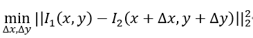
其中高斯牛顿法,即最小化灰度误差估计最优的像素偏移。在具体函数实现中(即calculateOpticalFlow),求解这样一个问题:
Opencv中的LK光流:使用 cv::calculateOpticalFlowPyrLK函数:
- 提供前后两张图像及对应的特征点,即可得到追踪后的点,以及各点的状态、误差;
- 根据status变量是否为1来确定对应的点是否被正确追踪到。
- cv::calcOpticalFlowPyrLK(img1,img2,pt1,pt2,status,error);
单层光流:用高斯牛顿法实现光流,光流也可以看成一个优化问题,通过最小化灰度误差估计最优的像素偏移
多层光流:因为单层光流在相机运动较快的情况下,容易达到一个局部极小值,因此引入图像金字塔。当原始图像的像素运动较大时,在金字塔顶层看来,运动仍然是一个小的运动范围
二、代码注释
#include<opencv2/opencv.hpp>
#include<string>
#include<chrono>
#include<Eigen/Core>
#include<Eigen/Dense>
using namespace std;
using namespace cv;
string file_1="./LK1.png"; //第一张图像的路径,可能需要写成绝对路径
string file_2="./LK2.png"; //第二张图像的路径
//使用高斯牛顿法实现光流
//定义一个光流追踪类
class OpticalFlowTracker
{
public:
OpticalFlowTracker( //带参构造函数,并初始化
const Mat &img1_,
const Mat &img2_,
const vector<KeyPoint>&kp1_,
vector<KeyPoint>&kp2_,
vector<bool>&success_,
bool inverse_=true,bool has_initial_=false):
img1(img1_),img2(img2_),kp1(kp1_),kp2(kp2_),success(success_),inverse(inverse_),
has_initial(has_initial_) {}
//计算光流的函数
void calculateOpticalFlow(const Range &range); //range是一个区间,应该看作一个窗口
private:
const Mat &img1;
const Mat &img2;
const vector<KeyPoint> &kp1;
vector<KeyPoint> &kp2;
vector<bool> &success;
bool inverse=true;
bool has_initial=false;
};
//单层光流的函数声明
void OpticalFlowSingleLevel(
const Mat &img1,
const Mat &img2,
const vector<KeyPoint>&kp1,
vector<KeyPoint>&kp2,
vector<bool>&success,
bool inverse=false,
bool has_initial_guess=false
);
//多层光流的函数声明
void OpticalFlowMultiLevel(
const Mat &img1,
const Mat &img2,
const vector<KeyPoint>&kp1,
vector<KeyPoint>&kp2,
vector<bool> &success,
bool inverse=false
);
//从图像中获取一个灰度值
//采用双线性内插法,来估计一个点的像素:
//f(x,y)=f(0,0)(1-x)(1-y)+f(1,0)x(1-y)+f(0,1)(1-x)y+f(1,1)xy
inline float GetPixelValue(const cv::Mat &img,float x,float y)
{
//边缘检测
if(x<0)
x=0;
if(y<0)
y=0;
if(x>=img.cols)
x=img.cols-1;
if(y>=img.rows)
y=img.rows-1;
uchar *data=&img.data[int(y)*img.step+int(x)]; //img.step:表示图像矩阵中每行包含的字节数;int(x)将x转换为int类型
float xx=x-floor(x); //floor(x)函数:向下取整函数,即返回一个不大于x的最大整数
float yy=y-floor(y);
return float(
(1-xx)*(1-yy)*data[0]+
xx*(1-yy)*data[1]+
(1-xx)*yy*data[img.step]+
xx*yy*data[img.step+1]
);
}
//主函数
int main(int argc,char**argv)
{
Mat img1=imread(file_1,0); //以灰度读取图像,重点
Mat img2=imread(file_2,0);
//特征点检测
vector<KeyPoint>kp1; //关键点 存放在容器kp1中
Ptr<GFTTDetector> detector=GFTTDetector::create(500,0.01,20); //通过GFTTD来获取角点,参数:最大角点数目500;角点可以接受的最小特征值0.01;角点之间的最小距离20
detector->detect(img1,kp1);//类似于ORB特征点的提取过程
//接下来实现在第二张图像中追踪这些角点,即追踪 kp1
//第一种方法:单层光流
vector<KeyPoint>kp2_single;
vector<bool>success_single;
OpticalFlowSingleLevel(img1,img2,kp1,kp2_single,success_single);
//第二种方法:多层光流
vector<KeyPoint>kp2_multi;
vector<bool>success_multi;
chrono::steady_clock::time_point t1=chrono::steady_clock::now();
OpticalFlowMultiLevel(img1,img2,kp1,kp2_multi,success_multi,true);
chrono::steady_clock::time_point t2=chrono::steady_clock::now();
auto time_used=chrono::duration_cast<chrono::duration<double>>(t2-t1);
//输出使用高斯牛顿法所花费的时间
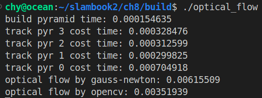
cout << "optical flow by gauss-newton: " << time_used.count() << endl;
//使用OpenCV中的LK光流
vector<Point2f>pt1,pt2;
for(auto &kp:kp1) //kp1中存放的是第一张图像中的角点,通过遍历,将kp1存放在pt1中
pt1.push_back(kp.pt);
vector<uchar>status;
vector<float>error;
t1=chrono::steady_clock::now();
//调用cv::calculateOpticalFlowPyrLK函数:
//提供前后两张图像及对应的特征点,即可得到追踪后的点,以及各点的状态、误差;
//根据status变量是否为1来确定对应的点是否被正确追踪到。
cv::calcOpticalFlowPyrLK(img1,img2,pt1,pt2,status,error);
t2=chrono::steady_clock::now();
time_used=chrono::duration_cast<chrono::duration<double>>(t2-t1);
cout << "optical flow by opencv: " << time_used.count() << endl; //输出使用opencv所花费的时间
//下面一部分代码实现绘图的功能
//第一张图像:单层光流的效果图
Mat img2_single;
//将输入图像从一个空间转换到另一个色彩空间
cv::cvtColor(img2,img2_single,CV_GRAY2BGR); //cvtColor()函数实现的功能:将img2灰度图转换成彩色图img2_single输出
for(int i=0;i<kp2_single.size();i++)
{
if(success_single[i]) //判断是否追踪成功
{
//circle():画圆:参数:源图像,画圆的圆心坐标,圆的半径,圆的颜色,线条的粗细程度
//kp2_single[i].pt:用来取第i个角点的坐标;Scalar(0,250,0):设置颜色,遵循B G R ,所以此图中为绿色
cv::circle(img2_single,kp2_single[i].pt,2,cv::Scalar(0,250,0),2);
//line():绘制直线:参数:要画的线所在的图像,直线起点,直线终点,直线的颜色(绿色)
cv::line(img2_single,kp1[i].pt,kp2_single[i].pt,cv::Scalar(0,250,0));
}
}
//第二张图像:多层光流的效果图
Mat img2_multi;
cv::cvtColor(img2,img2_multi,CV_GRAY2BGR);
for(int i=0;i<kp2_multi.size();i++)
{
if(success_multi[i])
{
cv::circle(img2_multi,kp2_multi[i].pt,2,cv::Scalar(250,0,0),2);
cv::line(img2_multi,kp1[i].pt,kp2_multi[i].pt,cv::Scalar(250,0,0));
}
}
//第三张图像:使用OpenCV中的LK光流
Mat img2_CV;
cv::cvtColor(img2,img2_CV,CV_GRAY2BGR);
for(int i=0;i<pt2.size();i++)
{
if(status[i])
{
cv::circle(img2_CV,pt2[i],2,cv::Scalar(0,0,250),2);
cv::line(img2_CV,pt1[i],pt2[i],cv::Scalar(0,0,250));
}
}
//
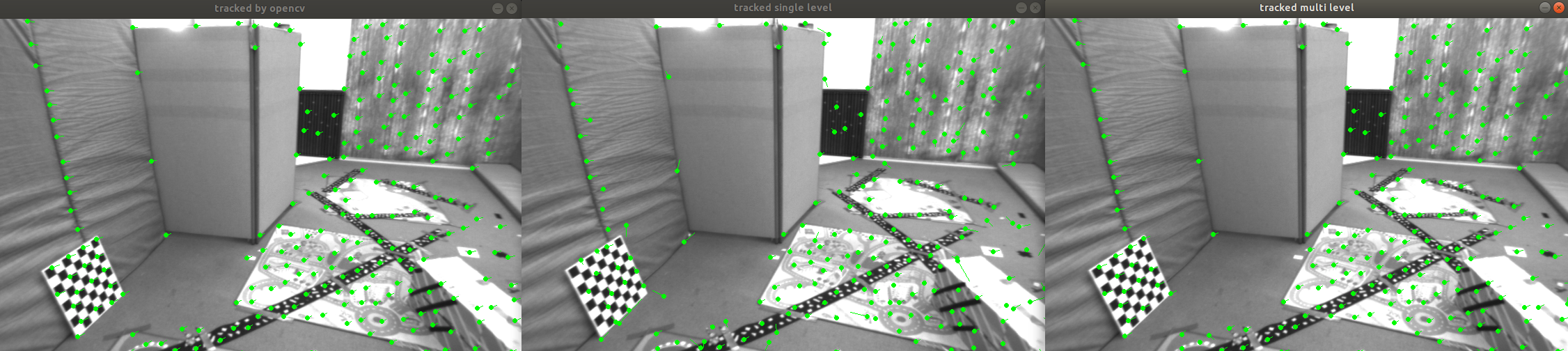
cv::imshow("tracked single level",img2_single);
cv::imshow("tracked multi level",img2_multi);
cv::imshow("tracked by opencv",img2_CV);
cv::waitKey(0);
return 0;
}具体功能实现如下:
 //接下来这一部分:具体函数的实现
 //第一个:单层光流函数的实现
 void OpticalFlowSingleLevel(
   const Mat &img1,
   const Mat &img2,
   const vector<KeyPoint>&kp1,
   vector<KeyPoint>&kp2,
   vector<bool>&success,
   bool inverse,
   bool has_initial)
 {
   //resize()函数:调整图像的大小;size()函数:获取kp1的长度
   //初始化
   kp2.resize(kp1.size());
   success.resize(kp1.size());   //是否追踪成功的标志

   OpticalFlowTracker tracker(img1,img2,kp1,kp2,success,inverse,has_initial);  //创建类的对象tracker
   //调用parallel_for_并行调用OpticalFlowTracker::calculateOpticalFlow,该函数计算指定范围内特征点的光流
   //range():从指定的第一个值开始,并在到达指定的第二个值后终止
   parallel_for_(Range(0,kp1.size()),std::bind(&OpticalFlowTracker::calculateOpticalFlow,&tracker,placeholders::_1));
 }

 //类外实现成员函数
 void OpticalFlowTracker::calculateOpticalFlow(const Range &range)
 {
   //定义参数
   int half_patch_size=4;  //窗口的大小8×8
   int iterations=10;  //每个角点迭代10次
   for(size_t i=range.start;i<range.end;i++)
   {
     auto kp=kp1[i];   //将第一张图像中的第i个关键点kp1[i]存放在 kp 中
     double dx=0,dy=0; //初始化
     if(has_initial)
     {
dx=kp2[i].pt.x-kp.pt.x;   //第i个点在第二张图像中的位置与第一张图像中的位置的差值
dy=kp2[i].pt.y-kp.pt.y;
     }

     double cost=0,lastCost=0;
     bool succ=true;

     //高斯牛顿方程
     //高斯牛顿迭代
     Eigen::Matrix2d H = Eigen::Matrix2d::Zero();   //定义H,并进行初始化。
     Eigen::Vector2d b = Eigen::Vector2d::Zero();   //定义b,并初始化.
     Eigen::Vector2d J;   //定义雅克比矩阵2×1
     for(int iter=0;iter<iterations;iter++)
     {
if(inverse==false)
{
  H=Eigen::Matrix2d::Zero();
  b=Eigen::Vector2d::Zero();
}
else
{
  b=Eigen::Vector2d::Zero();
}
cost=0;
//假设在这个8×8的窗口内像素具有同样的运动
//计算cost和J
for(int x=-half_patch_size;x<half_patch_size;x++)
  for(int y=-half_patch_size;y<half_patch_size;y++)
  {
    //GetPixelValue()计算某点的灰度值
    //计算残差:I(x,y)-I(x+dx,y+dy)
    double error=GetPixelValue(img1,kp.pt.x+x,kp.pt.y+y)-GetPixelValue(img2,kp.pt.x+x+dx,kp.pt.y+y+dy);;
    if(inverse==false)
    {
      //雅克比矩阵为第二个图像在x+dx,y+dy处的梯度
      J=-1.0*Eigen::Vector2d(0.5*(GetPixelValue(img2,kp.pt.x+dx+x+1,kp.pt.y+dy+y)-
                                 GetPixelValue(img2,kp.pt.x+dx+x-1,kp.pt.y+dy+y)),
			     0.5*(GetPixelValue(img2,kp.pt.x+dx+x,kp.pt.y+dy+y+1)-
			         GetPixelValue(img2,kp.pt.x+dx+x,kp.pt.y+dy+y-1)));
    }
    else if(iter==0)  //如果是第一次迭代,梯度为第一个图像的梯度,反向光流法
      //在反向光流中,I(x,y)的梯度是保持不变的,可以在第一次迭代时保留计算的结果,在后续的迭代中使用。
      //当雅克比矩阵不变时,H矩阵不变,每次迭代只需要计算残差。
    {
      J=-1.0*Eigen::Vector2d(0.5*(GetPixelValue(img1,kp.pt.x+x+1,kp.pt.y+y)-
                                 GetPixelValue(img1,kp.pt.x+x-1,kp.pt.y+y)),
			     0.5*(GetPixelValue(img1,kp.pt.x+x,kp.pt.y+y+1)-
			         GetPixelValue(img1,kp.pt.x+x,kp.pt.y+y-1)));
    }
    //计算H和b
    b+=-error*J;
    cost+=error*error;
    if(inverse==false||iter==0)
    {
      H+=J*J.transpose();
    }
  }
  //计算增量update,求解线性方程Hx=b
  Eigen::Vector2d update=H.ldlt().solve(b);
  if(std::isnan(update[0]))  //判断增量
  {
    //有时当我们遇到一个黑色或白色的方块,H是不可逆的,即高斯牛顿方程无解
    cout<<"update is nan"<<endl;
    succ=false;   //追踪失败
    break;
  }
  if(iter>0&&cost>lastCost)
  {
    break;
  }
  dx+=update[0];
  dy+=update[1];
  lastCost=cost;
  succ=true;
  if(update.norm()<1e-2)
  {
    break;
  }
     }
     success[i]=succ;
     kp2[i].pt=kp.pt+Point2f(dx,dy);
   }
 }//迭代完成

 //第二个:多层光流函数的实现
 void OpticalFlowMultiLevel(
   const Mat &img1,
   const Mat &img2,
   const vector<KeyPoint>&kp1,
   vector<KeyPoint>&kp2,
   vector<bool>&success,
   bool inverse)
 {
   int pyramids=4; //建立4层金字塔
   double pyramid_scale=0.5;  //金字塔每层缩小0.5
   double scales[]={1.0,0.5,0.25,0.125};

   //建立金字塔
   chrono::steady_clock::time_point t1=chrono::steady_clock::now();  //计算时间
   vector<Mat>pyr1,pyr2;
   for(int i=0;i<pyramids;i++)
   {
     if(i==0)
     {
//将两张图像存放在pyr1,pyr2中
pyr1.push_back(img1);
pyr2.push_back(img2);
     }
     else
     {
Mat img1_pyr,img2_pyr;
//对图像进行缩放,参数:原图,输出图像,输出图像大小,Size(宽度,高度)
cv::resize(pyr1[i-1],img1_pyr,cv::Size(pyr1[i-1].cols*pyramid_scale,pyr1[i-1].rows*pyramid_scale));
cv::resize(pyr2[i-1],img2_pyr,cv::Size(pyr2[i-1].cols*pyramid_scale,pyr2[i-1].rows*pyramid_scale));
pyr1.push_back(img1_pyr);
pyr2.push_back(img2_pyr);
     }
   }
   chrono::steady_clock::time_point t2=chrono::steady_clock::now();
   auto time_used=chrono::duration_cast<chrono::duration<double>>(t2-t1);
   cout<<"build pyramid time:"<<time_used.count()<<endl;

   //计算光流时,先从顶层的图像开始计算
   vector<KeyPoint>kp1_pyr,kp2_pyr;
   for(auto &kp:kp1)
   {
     auto kp_top=kp;
     kp_top.pt *=scales[pyramids-1];   //顶层
     kp1_pyr.push_back(kp_top);
     kp2_pyr.push_back(kp_top);
   }

   for(int level=pyramids-1;level>=0;level--)
   {
     success.clear();
     t1=chrono::steady_clock::now();
     OpticalFlowSingleLevel(pyr1[level],pyr2[level],kp1_pyr,kp2_pyr,success,inverse,true);
     t2=chrono::steady_clock::now();
     auto time_used=chrono::duration_cast<chrono::duration<double>>(t2-t1);
     cout<<"track pyr"<<level<<"cost time:"<<time_used.count()<<endl;
     if(level>0)
     {
for(auto &kp:kp1_pyr)
  kp.pt/=pyramid_scale;
for(auto &kp:kp2_pyr)
  kp.pt/=pyramid_scale;
     }
   }
   for(auto &kp:kp2_pyr)
     kp2.push_back(kp);
 }
ch8/direct_method.cpp
在光流中,我们会首先追踪特征点的位置,再根据这些位置确定相机的运动。这样一种两步走的方案,很难保证全局最优。直接法通过在后一步中调整前一步的结果
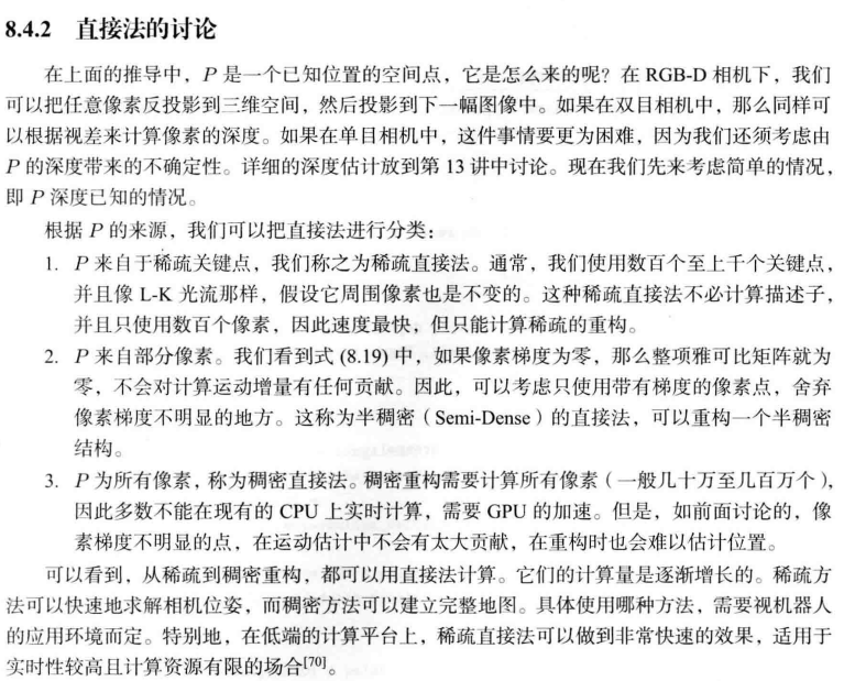
代码注释待更新~~~~